【3】16S rRNA 菌叢解析やってみた(visualization of taxonomy abundance, α,β-diversity by MicrobiotaProcess)
こんにちは~。ガイです。
前回、前々回で生データ処理~分類群情報とその頻度を取得するところまで終わりました。ここからはいよいよ様々な指標の可視化に入っていきます。
ブログを見ている人にはお察しかもしれませんが、わたしはR スキルがあまりありません。なので、データの可視化にあたって、自力で見栄えのいい図を作ることは端から諦め、インターネットの海の中、見栄えのいい図を作ってくれるソフトウェアを探し回りました。そこでたどり着いたのがMicrobiotaProcess です。
MicrobiotaProcess は微生物データセットの解析、可視化、バイオマーカー探索のためのRパッケージです。わたしの目的にぴったりのソフトウェアでした。
Xu S, Zhan L, Tang W, Wang Q, Dai Z, Zhou L, Feng T, Chen M, Wu T, Hu E, Yu G (2023). “MicrobiotaProcess: A comprehensive R package for deep mining microbiome.” The Innovation, 4, 100388. ISSN 2666-6758, doi:10.1016/j.xinn.2023.100388, https://www.sciencedirect.com/science/article/pii/S2666675823000164.
ということで、今回はMicrobiotaProcess を使ったデータの可視化をチュートリアルに基本的には従って行っていきたいと思います。自分なりの工夫を入れている箇所は赤字にしてあります。あと、「おまけ」と書いてあるところはわたしが自分の趣味でやったところです。
どこぞの大学院生のブログよりチュートリアル原文の方が信用できるわい!という人は以下のページからどうぞ。
- 多様性解析用系統樹の作成
- MicrobiotaProcess のインストール
- インプットファイルの読み込み
- MicrobiotaProcess に必要なパッケージ
- alpha diversity analysis
- The visualization of taxonomy abundance
- Beta diversity analysis
- Biomarker discovery
- mp_diff_analysis
多様性解析用系統樹の作成
解析を始める前に、ひとつ忘れていたことがありました。解析用の系統樹の作成です。“Moving Pictures” tutorial を参考に作っておきます。
参考:Generate a tree for phylogenetic diversity analyses “Moving Pictures” tutorial — QIIME 2 2023.2.0 documentation
qiime phylogeny align-to-tree-mafft-fasttree \
  --i-sequences rep-seqs.qza \
  --o-alignment aligned-rep-seqs.qza \
  --o-masked-alignment masked-aligned-rep-seqs.qza \
  --o-tree unrooted-tree.qza \
  --o-rooted-tree rooted-tree.qza
MicrobiotaProcess のインストール
まずRを起動します。つぎに、公式ページに従って以下を実行。
参考:Bioconductor - MicrobiotaProcess
if (!require("BiocManager", quietly = TRUE))
install.packages("BiocManager")
BiocManager::install("MicrobiotaProcess")
インプットファイルの読み込み
以下のページに様々な形式のデータからのMPSE object としての読み込み方法が乗っています。
3.1 bridges other tools https://bioconductor.org/packages/devel/bioc/vignettes/MicrobiotaProcess/inst/doc//MicrobiotaProcess.html#bridges-other-tools
【2024/08/08 修正】以前やっていた方法でインプットを取り込むとのちのち警告が出るので取り込み方を変えました。
修正版MPSE 変換方法
必要なパッケージの読み込み
library(qiime2R)
library(tidyverse)
library(phyloseq)
library(MicrobiotaProcess)
インプットファイルの変換
# parsing the output of qiime2
otuqzafile <- "~/path/to/selected_table.qza" # テーブルの読み込み(リード数によるセレクションなどかけていない場合はtable.qza)
taxaqzafile <- ("~/path/to/taxonomy.qza") # 系統アノテーションの読み込み
mapfile <- "~/path/to/METADATA.tsv" # メタデータの読み込み
treefile = "~/path/to/rooted-tree.qza" # 系統樹の読み込み

mpse <- mp_import_qiime2(otuqza=otuqzafile, taxaqza=taxaqzafile, mapfilename=mapfile, treeqza = treefile)
【以前やっていた方法】
わたしはここに載っている方法を色々試して上手くいかなかったので、Qiita 記事(https://t.co/MpfAAYmeWf)を参考にしてphyloseq 形式でデータを読み込んだ後でMPSE 形式に変換しました。が、Qiita ページが削除されてしまっているようです。残念です。
まず、QIIME2R, dplyr, phyloseq パッケージをインストールし、読み込みます。
# QIIME2R install
if (!requireNamespace("devtools", quietly = TRUE)){install.packages("devtools")}
devtools::install_github("jbisanz/qiime2R")
library(qiime2R)

# dplyr install
install.packages(“dplyr”)
library(dplyr)

# phyloseq install
if(!requireNamespace("BiocManager")){
  install.packages("BiocManager")
}
BiocManager::install("phyloseq")
library(phyloseq)
つぎにファイルの読み込み。
# データのインポート
tree <- qiime2R::read_qza("~/path/to/rooted-tree.qza") # 系統樹の読み込み
otus <-qiime2R::read_qza("~/path/to/selected_table.qza") # テーブルの読み込み(リード数によるセレクションなどかけていない場合はtable.qza)
taxonomy <- qiime2R::read_qza("~/path/to/taxonomy.qza") # 系統アノテーションの読み込み
repseq <- qiime2R::read_qza("~/path/to/rep-seqs.qza") # 代表配列の読み込み
tax_table <- parse_taxonomy(taxonomy$data)
tax_table <- as.matrix(tax_table)
metadata <- read.table("METADATA.LHR.tsv", sep = "\t", header=T,
                         row.names=1) %>% sample_data() # メタデータの読み込み

ps <- phyloseq(otus = otu_table(otus$data, taxa_are_rows = T), tree = tree$data, tax_table = tax_table(tax_table), metadata = metadata, refseq = repseq$data) # phyloseq データに格納
# MicrobiotaProcess データ形式に変換
mpse <- ps %>% as.MPSE()
以下は必要ならやっておくといいです
# ASV名を変更しておきたい場合(図中に配列ID を表示したくない場合)
taxa_names(physeq) <- paste("ASV", order(order(rowSums(otu_table(physeq)), decreasing = T)), sep="")

# METADATA 内の要素の図示順を変えたいとき
## 以下の例では、Wild グループを先に図示し、HAPPY グループを後に図示したい場合です
 # factorの要素の新しい順序を定義する
 new_order <- c("Wild", "HAPPY")  # 新しい順序に合わせて要素を指定してください
 # サンプルデータフレームにアクセスする
  # phyloseq データの場合
 ps@sam_data$groups <- factor(ps@sam_data$groups, levels = new_order)
 # MPSE データの場合
 mpse@colData@listData$groups <- factor(mpse@colData@listData$groups, levels = new_order)
ここまではわたし自身のデータでやった場合の取り込み方法でしたが、ここからは自分のデータだとブログ等に貼り付けづらいので、以下のダウンロードデータで進めます。
https://www.microbiomeanalyst.ca/MicrobiomeAnalyst/resources/data/ibd_data.zip
wget https://www.microbiomeanalyst.ca/MicrobiomeAnalyst/resources/data/ibd_data.zip
unzip ibd_data.zip
中身です。
Archive:  ibd_data.zip
   creating: ibd_data/
   creating: ibd_data/IBD_data/
  inflating: ibd_data/IBD_data/ibd_meta.csv
  inflating: ibd_data/IBD_data/ibd_taxa.txt
  inflating: ibd_data/IBD_data/ibd_tsea_list.txt
  inflating: ibd_data/IBD_data/ibd_tree.tre
  inflating: ibd_data/IBD_data/ibd_asv_table.txt
以下に示すibd_meta.csv の中身を見るとわかりますが、今回のグループ分けの名称はClass、各グループ名はCD とControl で、sample ID が6 桁の数字になります。チュートリアルで使われているデータとグループ名が異なるので、その点は各スクリプトにおいて修正しています(time →Class)。また、格納データ名もチュートリアルではmouse.time.mpse ですが、わたしはmpse という名前を付けています。
> ibd_meta.csv
#NAME,Class
206700,CD
206701,CD
206702,CD
206703,Control
206704,Control
(以下略)

> ibd_taxa.txt
#TAXONOMY    Kingdom    Phylum    Class    Order    Family    Genus    Species
TACGGAGGATCCGAGCGTTATCCGGATTTATTGGGTTTAAAGGGAGCGTAGATGGATGTTTAAGTCAGTTGTGAAAGTTTGCGGCTCAACCGTAAAATTGCAGTTGATACTGGATATCTTGAGTGCAGTTGAGGCAGGCGGAATTCGTGGTGTAGCGGTGAAATGCTTAGATATCACGAAGAACTCCGATTGCGAAGGCAGCCTGCTAAGCTGCAACTGACATTGAGGCTCGAAAGTGTGGGTATCAAACAGG    k__Bacteria    p__Bacteroidetes    c__Bacteroidia    o__Bacteroidales    f__Bacteroidaceae    g__Bacteroides    s__
AACGTAGGTCACAAGCGTTGTCCGGAATTACTGGGTGTAAAGGGAGCGCAGGCGGGAAGACAAGTTGGAAGTGAAATCTATGGGCTCAACCCATAAACTGCTTTCAAAACTGTTTTTCTTGAGTAGTGCAGAGGTAGGCGGAATTCCCGGTGTAGCGGTGGAATGCGTAGATATCGGGAGGAACACCAGTGGCGAAGGCGGCCTACTGGGCACCAACTGACGCTGAGGCTCGAAAGTGTGGGTAGCAAACAGG    k__Bacteria    p__Firmicutes    c__Clostridia    o__Clostridiales    f__Ruminococcaceae    g__Faecalibacterium    s__prausnitzii
(以下略)

> ibd_asv_table.txt
#NAME    206700    206701    206702    206703    206704    206708    206709    206710    206711    206718    206719    206720    206721    206725    206726    206727    206728    206734    206738    206739    206740    206741    206742    206743    206750    206751    206756    206767    206768    215075    219633    219634    219651    219652    219655    219656    219659    219675    219691    224323    224324    224327    224328
TACGGAGGATCCGAGCGTTATCCGGATTTATTGGGTTTAAAGGGAGCGTAGATGGATGTTTAAGTCAGTTGTGAAAGTTTGCGGCTCAACCGTAAAATTGCAGTTGATACTGGATATCTTGAGTGCAGTTGAGGCAGGCGGAATTCGTGGTGTAGCGGTGAAATGCTTAGATATCACGAAGAACTCCGATTGCGAAGGCAGCCTGCTAAGCTGCAACTGACATTGAGGCTCGAAAGTGTGGGTATCAAACAGG    18    53    55    8638    4154    11997    18174    10334    10295    0    25    5871    5449    13262    18084    5995    4458    21    0    0    4919    6761    5663    6975    9447    7915    13850    6573    7    18451    463    291    2104    2129    1037    881    377    1913    0    7713    12094    10241    11611
AACGTAGGTCACAAGCGTTGTCCGGAATTACTGGGTGTAAAGGGAGCGCAGGCGGGAAGACAAGTTGGAAGTGAAATCTATGGGCTCAACCCATAAACTGCTTTCAAAACTGTTTTTCTTGAGTAGTGCAGAGGTAGGCGGAATTCCCGGTGTAGCGGTGGAATGCGTAGATATCGGGAGGAACACCAGTGGCGAAGGCGGCCTACTGGGCACCAACTGACGCTGAGGCTCGAAAGTGTGGGTAGCAAACAGG    10    0    0    979    1675    8346    7125    8242    6844    4865    6233    1085    561    12258    8590    13890    16880    344    4558    6297    3518    2932    3095    1102    2824    2582    1699    1506    0    7751    3239    1735    3023    3170    637    407    192    0    3294    5118    3815    5707    5745

> ibd_tree.tre
(TACGTAGGGGGC(中略)CAAACAGG:1e-08,((((TACGTATGGTGCAAGCGTTATCCGGATTTACTGGGTGTAAAGGGAGCGTAGACGGTAAAGCAAGTCTGAAGTGAAAGCCCGGGGCTCAACC(中略)CTTACTGGACAGTAACTGACGTTGAGGCTCGAAAGCGTGGGGAGCAAACAGG:1e-08,(TAC(以下略)
ダウンロードデータの読み込み
ほぼ以下の公式チュートリアル通りですが、赤字のところだけエラーが出るので変えています。
公式:Workshop of microbiome dataset analysis using MicrobiotaProcess • MicrobiotaProcessWorkshop
library(MicrobiotaProcess)
library(phyloseq)

otuda <- read.table("~/path_to/ibd_data/IBD_data/ibd_asv_table.txt", header=T, check.names=F, comment.char="", row.names=1, sep="\t")
# building the output format of removeBimeraDenovo of dada2
otuda <- data.frame(t(otuda), check.names=F)
sampleda <- read.csv("~/path_to/ibd_data/IBD_data/ibd_meta.csv", row.names=1, comment.char="")
taxda <- read.table("~/path_to/ibd_data/IBD_data/ibd_taxa.txt", header=T, row.names=1, check.names=F, comment.char="")
# the feature names should be the same with rownames of taxda.
taxda <- taxda[match(colnames(otuda), rownames(taxda)),]
tree <- read_tree(treefile = "path_to/ibd_data/IBD_data/ibd_tree.tre")

psraw <- import_dada2( seqtab = otuda, taxatab = taxda, reftree = tree, sampleda = sampleda, btree = FALSE )
# view the reads depth of samples. In this example,
# we remove the sample contained less than 20914 otus.
# sort(rowSums(otu_table(psraw)))
# samples were removed, which the reads number is too little.
psraw <- prune_samples(sample_sums(psraw)>=sort(rowSums(otu_table(psraw)))[3], psraw)
# then the samples were rarefied to 20914 reads.
set.seed(1024)
ps <- rarefy_even_depth(psraw)
mpse <- ps %>% as.MPSE()
MicrobiotaProcess に必要なパッケージ
すみません。いちいちインストールの話からするのがめんどうになってきたので、必要なパッケージをあげておきます。インストールしておいてください。
公式チュートリアルに載っているパッケージ
library(MicrobiotaProcess)
# an R package for analysis, visualization and biomarker discovery of Microbiome.
library(phyloseq) # Handling and analysis of high-throughput microbiome census data.
library(ggplot2) # Create Elegant Data Visualisations Using the Grammar of Graphics.
library(tidyverse) # Easily Install and Load the 'Tidyverse'.
library(vegan) # Community Ecology Package.
library(coin) # Conditional Inference Procedures in a Permutation Test Framework.
library(reshape2) # Flexibly Reshape Data: A Reboot of the Reshape Package.
library(ggnewscale) # Multiple Fill and Colour Scales in 'ggplot2'.
公式チュートリアルに載っていないがおそらく必要になってくるパッケージ(解析による)
library(shadowtext)
library(qiime2R)
library(gghalves)
library(ggalluvial)
library(corrr)
library(ggh4x)
library(ggside)
alpha diversity analysis
Rarefaction visualization
何リード以上でα 多様性がプラトーに達するのか調べます。
なぜこれが必要かは以下の資料がわかりやすいです。
井上亮. (2019). 腸内細菌叢解析のいろは. 日本乳酸菌学会誌, 30(1), 27-31.
https://www.jstage.jst.go.jp/article/jslab/30/1/30_27/_pdf
library(ggplot2)
library(MicrobiotaProcess)
# Rarefied species richness
mpse %<>% mp_rrarefy()
mpse %<>% mp_cal_rarecurve( .abundance = RareAbundance, chunks = 400 )
# サンプルの総リード数が40000である場合、chunksが400であれば、100のサブサンプル (100, 200, 300,..., 40000)に分割され、そのサブサンプルに基づいてアルファ多様性インデックスが計算される
mpse %>% print(width=180) # 結果の表示
作図
p1 <- mpse %>% mp_plot_rarecurve( .rare = RareAbundanceRarecurve, .alpha = Observe, )

p2 <- mpse %>% mp_plot_rarecurve( .rare = RareAbundanceRarecurve, .alpha = "ACE", .group = Class ) + scale_color_manual(values=c("#00A087FF", "#3C5488FF")) + scale_fill_manual(values=c("#00A087FF", "#3C5488FF"), guide="none")

# combine the samples belong to the same groups if  plot.group=TRUE
p3 <- mpse %>% mp_plot_rarecurve( .rare = RareAbundanceRarecurve, .alpha = "Chao1", .group = Class, plot.group = TRUE ) + scale_color_manual(values=c("#00A087FF", "#3C5488FF")) + scale_fill_manual(values=c("#00A087FF", "#3C5488FF"),guide="none")

# 図の保存
ggsave("rarecurve.pdf", plot = p1 + p2 + p3, dpi = 100, width = 16, height = 5, limitsize = FALSE)

Calculate alpha index and visualization
いよいよα 多様性の計算に入っていきます。
mp_cal_alpha コマンドを使用します。
# パッケージの読み込み
library(ggplot2)
library(MicrobiotaProcess)

# mp_cal_alpha コマンドによるα多様性指数の計算
mpse %<>% mp_cal_alpha(.abundance=RareAbundance)

# 結果
mpse
# A MPSE-tibble (MPSE object) abstraction: 53,793 × 18
# OTU=1251 | Samples=43 | Assays=Abundance, RareAbundance | Taxonomy=Kingdom,
# Phylum, Class, Order, Family, Genus, Species
OTU Sample Abundance RareAbundance Class RareAbundanceRarecurve Observe
<chr> <chr> <dbl> <dbl> <chr> <list> <dbl>
1 OTU_1207 206700 0 0 CD <tibble [2,574 × 4]> 72
2 OTU_1249 206700 0 0 CD <tibble [2,574 × 4]> 72
3 OTU_12 206700 145 145 CD <tibble [2,574 × 4]> 72
4 OTU_770 206700 0 0 CD <tibble [2,574 × 4]> 72
5 OTU_1107 206700 0 0 CD <tibble [2,574 × 4]> 72
6 OTU_46 206700 0 0 CD <tibble [2,574 × 4]> 72
7 OTU_343 206700 0 0 CD <tibble [2,574 × 4]> 72
8 OTU_601 206700 0 0 CD <tibble [2,574 × 4]> 72
9 OTU_971 206700 0 0 CD <tibble [2,574 × 4]> 72
10 OTU_135 206700 0 0 CD <tibble [2,574 × 4]> 72
# ℹ 53,783 more rows
# ℹ 11 more variables: Chao1 <dbl>, ACE <dbl>, Shannon <dbl>, Simpson <dbl>,
# Pielou <dbl>, Kingdom <chr>, Phylum <chr>, Order <chr>, Family <chr>,
# Genus <chr>, Species <chr>
# ℹ Use `print(n = ...)` to see more rows
図示
f1 <- mpse %>%
mp_plot_alpha(
             .group=Class,
             .alpha=c(Observe, Chao1, ACE, Shannon, Simpson, Pielou)
              ) +
             scale_fill_manual(values=c("#00A087FF", "#3C5488FF"), guide="none") +
             scale_color_manual(values=c("#00A087FF", "#3C5488FF"), guide="none")

f2 <- mpse %>%
 mp_plot_alpha(
.alpha=c(Observe, Chao1, ACE, Shannon, Simpson, Pielou)
               )

# ここで「loadNamespace(x) でエラー: ‘gghalves’ という名前のパッケージはありません」というエラーが出る可能性があります
# その場合にはあわてず騒がすインストールしてください
if (!require(devtools)) { install.packages('devtools') }
devtools::install_github('erocoar/gghalves')

# 図の保存
ggsave("alpha-diversity.pdf", plot = f1 / f2, dpi = 100, width = 16, height = 9, limitsize = FALSE)

The visualization of taxonomy abundance
生物群集の組成を計算、プロットしていきます。
生物群集の組成の計算
mp_cal_abundance コマンドで各サンプルまたはグループの各分類群の(相対)存在量を計算します。
mp_extract_abundance は特定の分類レベルの存在量を抽出することができます。存在量テーブルを抽出して、手動で可視化するなどの外部分析を行うこともできます(mp_cal_abundance)。
mpse %<>% mp_cal_abundance( .abundance = RareAbundance ) %>% mp_cal_abundance( .abundance=RareAbundance, .group=Class )

# 結果
mpse
# A MPSE-tibble (MPSE object) abstraction: 53,793 × 19
# OTU=1251 | Samples=43 | Assays=Abundance, RareAbundance,
# RelRareAbundanceBySample | Taxonomy=Kingdom, Phylum, Class, Order, Family,
# Genus, Species
OTU Sample Abundance RareAbundance RelRareAbundanceBySample Class
<chr> <chr> <dbl> <dbl> <dbl> <chr>
1 OTU_1207 206700 0 0 0 CD
2 OTU_1249 206700 0 0 0 CD
3 OTU_12 206700 145 145 3.76 CD
4 OTU_770 206700 0 0 0 CD
5 OTU_1107 206700 0 0 0 CD
6 OTU_46 206700 0 0 0 CD
7 OTU_343 206700 0 0 0 CD
8 OTU_601 206700 0 0 0 CD
9 OTU_971 206700 0 0 0 CD
10 OTU_135 206700 0 0 0 CD
# ℹ 53,783 more rows
# ℹ 13 more variables: RareAbundanceRarecurve <list>, Observe <dbl>,
# Chao1 <dbl>, ACE <dbl>, Shannon <dbl>, Simpson <dbl>, Pielou <dbl>,
# Kingdom <chr>, Phylum <chr>, Order <chr>, Family <chr>, Genus <chr>,
# Species <chr>
# ℹ Use `print(n = ...)` to see more rows
図示その1:サンプルごとのボックスプロット
# visualize the relative abundance of top 20 phyla for each sample.
p1 <- mpse %>% mp_plot_abundance( .abundance=RareAbundance, .group=Class, taxa.class = Phylum, topn = 20, relative = TRUE )
# visualize the abundance (rarefied) of top 20 family for each sample.
p2 <- mpse %>% mp_plot_abundance( .abundance=RareAbundance, .group=Class, taxa.class = Family, topn = 20, relative = FALSE )

# 図の保存
ggsave("taxonomy_Abundance.pdf", plot = p1 / p2, dpi = 100, width = 16, height = 9, limitsize = FALSE)

# わたしの場合、「xidx_w でエラー: レベル 2 にはそのようなインデックスはありません」 というエラーが出て進めなくなったのですがggalluvial とggh4x をconda で入れたら直りました

図示その2:グループごとのボックスプロット

# visualize the relative abundance of top 20 phyla for each .group (time)
p3 <- mpse %>% mp_plot_abundance( .abundance=RareAbundance, .group=Class, taxa.class = Phylum, topn = 20, plot.group = TRUE )

# visualize the abundance of top 20 phyla for each .group (time)
p4 <- mpse %>% mp_plot_abundance( .abundance=RareAbundance, .group= Class, taxa.class = Order, topn = 20, relative = FALSE, plot.group = TRUE )

# 図の保存
ggsave("groups_Abundance.pdf", plot = p3 / p4, dpi = 100, width = 16, height = 9, limitsize = FALSE)
図示その3:ヒートマップ
h1 <- mpse %>% mp_plot_abundance( .abundance = RareAbundance, .group = Class, taxa.class = Phylum, relative = TRUE, topn = 20, geom = 'heatmap', feature.dist = 'euclidean', feature.hclust = 'average', sample.dist = 'bray', sample.hclust = 'average' )
h2 <- mpse %>% mp_plot_abundance( .abundance = RareAbundance, .group = Class, taxa.class = Order, relative = FALSE, topn = 20, geom = 'heatmap', feature.dist = 'euclidean', feature.hclust = 'average', sample.dist = 'bray', sample.hclust = 'average' )

# 赤字の部分、公式チュートリアルが間違えていたので直しています
# チュートリアルのままやると「警告メッセージ: ggplot2::geom_tile(data = td_filter(!!rlang::sym(abundance.nm) !=  で: Ignoring unknown parameters: `features.dist` and `features.hclust` 警告メッセージ: ggplot2::geom_tile(data = td_filter(!!rlang::sym(abundance.nm) !=  で: Ignoring unknown parameters: `features.dist` and `features.hclust`」という警告が出ます。
# 正しくは以下:https://rdrr.io/github/xiangpin/MicrobitaProcess/man/mp_plot_abundance-methods.html
# 修正features.dist → feature.dist features.hclust → feature.hclust
# the character (scale or theme) of figure can be adjusted by set_scale_theme
# refer to the mp_plot_dist
plot <- aplot::plot_list(gglist=list(h1, h2), tag_levels="A")

# 図の保存
ggsave("heatmap_Abundance.pdf", plot = plot, dpi = 100, width = 16, height = 5, limitsize = FALSE)
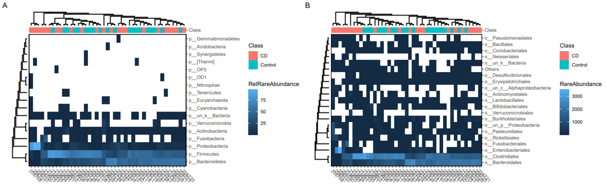

一部オプションの説明
|
Beta diversity analysis
グループ間距離を算出
# データの正規化 standardization (参考:https://rdrr.io/github/YuLab-SMU/MicrobiotaProcess/man/mp_decostand-methods.html)
# デフォルトはhellingerで、処理された存在量はassaysスロットに格納される
# 正規化メソッドは'total'、'max'、'frequency'、'normalize'、'range'、'rank'、'standardize'、'pa'、'chi.square'、'hellinger'、'log'のいずれかを指定
mpse %<>% mp_decostand(.abundance=Abundance)
# 結果
mpse
# A MPSE-tibble (MPSE object) abstraction: 53,793 × 20
# OTU=1251 | Samples=43 | Assays=Abundance, RareAbundance,
# RelRareAbundanceBySample, hellinger | Taxonomy=Kingdom, Phylum, Class,
# Order, Family, Genus, Species
OTU Sample Abundance RareAbundance RelRareAbundanceBySa…¹ hellinger Class
<chr> <chr> <dbl> <dbl> <dbl> <dbl> <chr>
1 OTU_12… 206700 0 0 0 0 CD
2 OTU_12… 206700 0 0 0 0 CD
3 OTU_12 206700 145 145 3.76 0.194 CD
4 OTU_770 206700 0 0 0 0 CD
5 OTU_11… 206700 0 0 0 0 CD
6 OTU_46 206700 0 0 0 0 CD
7 OTU_343 206700 0 0 0 0 CD
8 OTU_601 206700 0 0 0 0 CD
9 OTU_971 206700 0 0 0 0 CD
10 OTU_135 206700 0 0 0 0 CD
# ℹ 53,783 more rows
# ℹ abbreviated name: ¹RelRareAbundanceBySample
# ℹ 13 more variables: RareAbundanceRarecurve <list>, Observe <dbl>,
# Chao1 <dbl>, ACE <dbl>, Shannon <dbl>, Simpson <dbl>, Pielou <dbl>,
# Kingdom <chr>, Phylum <chr>, Order <chr>, Family <chr>, Genus <chr>,
# Species <chr>
# ℹ Use `print(n = ...)` to see more rows
サンプル間距離の算出
# サンプル間の距離を算出
mpse %<>% mp_cal_dist(.abundance=hellinger, distmethod="bray")

# distmethod で距離の計算方法を指定(参考:https://rdrr.io/github/YuLab-SMU/MicrobiotaProcess/man/mp_cal_dist-methods.html)
# オプションはかなり豊富にある("maximum", "binary", "minkowski" (implemented in dist of stats), "unifrac" ほか)
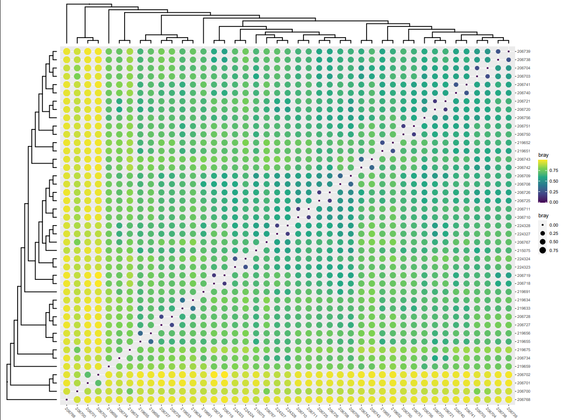
サンプル間距離の可視化
p1 <- mpse %>% mp_plot_dist(.distmethod = bray)

# 図の保存
ggsave("samples_beta.pdf", plot = p1, dpi = 100, width = 16, height = 12, limitsize = FALSE)
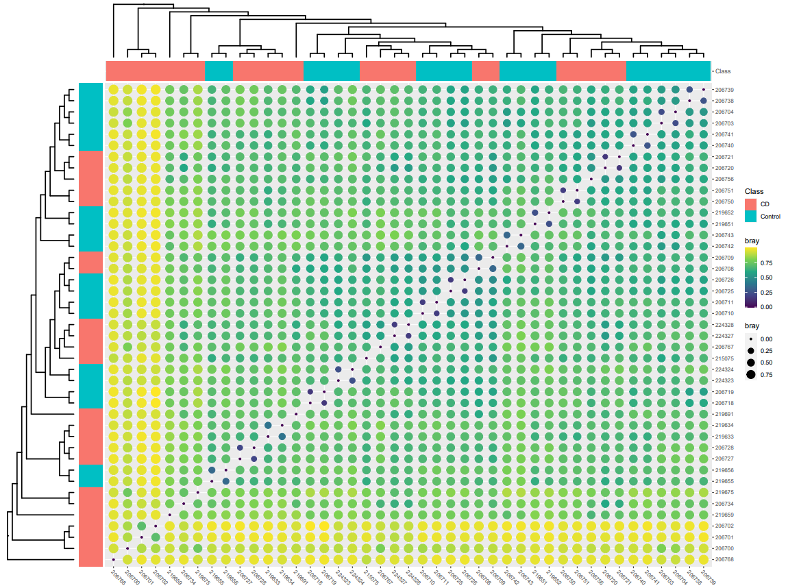
グループ間距離の可視化
# when .group is provided, the dot heatmap plot with group information will be return.
p2 <- mpse %>% mp_plot_dist(.distmethod = bray, .group = Class)

# The scale or theme of dot heatmap plot can be adjusted using set_scale_theme function.

p2 %>% set_scale_theme( x = scale_fill_manual( values=c("orange", "deepskyblue"), guide = guide_legend( keywidth = 1, keyheight = 0.5, title.theme = element_text(size=8), label.theme = element_text(size=6)改 ) ), aes_var = time # specific the name of variable ) %>% set_scale_theme( x = scale_color_gradient( guide = guide_legend(keywidth = 0.5, keyheight = 0.5) ), aes_var = bray ) %>% set_scale_theme( x = scale_size_continuous( range = c(0.1, 3), guide = guide_legend(keywidth = 0.5, keyheight = 0.5) ), aes_var = bray )

# 図の保存
ggsave("groups_beta.pdf", plot = p2, dpi = 100, width = 16, height = 12, limitsize = FALSE)
グループ間およびグループ内距離の有意差検定
# group.test=TRUE により、検定が実行される。
# デフォルトはwilcox.test
# 変更にはtest オプションを使用する
# 検定の種類について説明が見つけられないが、ほかのコマンドと同じであるならば ’wilcox_test’ of ’coin’; ’glm’; ’glm.nb’ of ’MASS'
# 参考:https://bioc.ism.ac.jp/packages/devel/bioc/manuals/MicrobiotaProcess/man/MicrobiotaProcess.pdf
# 図示
p3 <- mpse %>% mp_plot_dist(.distmethod = bray, .group = Class, group.test=TRUE, textsize=2)

# 図の保存
ggsave("groups_beta_stat.pdf", plot = p3, dpi = 100, width = 16, height = 12, limitsize = FALSE)

The PCoA analysis
PCoA により距離の可視化を行います。
mpse %<>% mp_cal_pcoa(.abundance=hellinger, distmethod="bray")
# 順序分析の次元は、デフォルトでcolData スロットに追加される

# また、アドニス(adonis)やアノシム(anosim)を実行してグループの非類似性が有意かどうかをチェックすることもできる。
# adonis とはvegan パッケージに入っているPERMANOVA 用関数
# 参考1:https://rdrr.io/github/YuLab-SMU/MicrobiotaProcess/man/mp_adonis-methods.html
# 参考2:土居秀幸, & 岡村寛. (2011). 生物群集解析のための類似度とその応用: R を使った類似度の算出, グラフ化, 検定. 日本生態学会誌, 61(1), 3-20.https://www.jstage.jst.go.jp/article/seitai/61/1/61_KJ00007176266/_pdf
mpse %<>% mp_adonis(.abundance=hellinger, .formula=~Class, distmethod="bray", permutations=9999, action="add")

The result of adonis has been saved to the internal attribute !
It can be extracted using this-object %>% mp_extract_internal_attr(name='adonis')

# 結果をmpse データに追加
mpse %>% mp_extract_internal_attr(name=adonis)

# 結果が表示される
The object contained internal attribute: PCoA ADONIS
Permutation test for adonis under reduced model
Terms added sequentially (first to last)
Permutation: free
Number of permutations: 9999
vegan::adonis2(formula = .formula, data = sampleda, permutations = permutations, method = distmethod)
         Df SumOfSqs     R2      F Pr(>F)
Class     1   0.8119 0.0723 3.1955  1e-04 ***
Residual 41  10.4173 0.9277
Total    42  11.2292 1.0000
---
Signif. codes:  0 ‘***’ 0.001 ‘**’ 0.01 ‘*’ 0.05 ‘.’ 0.1 ‘ ’ 1
PCoA 結果の図示
library(ggplot2)

p1 <- mpse %>% mp_plot_ord( .ord = pcoa, .group = Class, .color = Class, .size = 1.2, .alpha = 1, ellipse = TRUE, show.legend = FALSE )

p2 <- mpse %>% mp_plot_ord( .ord = pcoa, .group = Class, .color = Class, .size = Observe, .alpha = Shannon, ellipse = TRUE, show.legend = FALSE )

# 図の保存
ggsave("PCoA.pdf", plot = p1 + p2, dpi = 100, width = 16, height = 5, limitsize = FALSE)

おまけ weighted unifrac のPCoA グラフを書き、bray のグラフと並べて図示したい
ちなみに、weighted unifracはmp_cal_distオプションがないっぽいのであきらました。
# The distance between samples or groups
mpse %<>% mp_decostand(.abundance=Abundance)

# unifrac
mpse_uni <- mpse
mpse_uni %<>% mp_cal_dist(.abundance=hellinger, distmethod="unifrac")
mpse_uni %<>% mp_cal_pcoa(.abundance=hellinger, distmethod="unifrac")
mpse_uni %<>% mp_adonis(.abundance=hellinger, .formula=~Class, distmethod="unifrac", permutations=9999, action="add")
mpse_uni %>% mp_extract_internal_attr(name=adonis)

#結果
The result of adonis has been saved to the internal attribute !
It can be extracted using this-object %>% mp_extract_internal_attr(name='adonis')
The object contained internal attribute: PCoA ADONIS
Permutation test for adonis under reduced model
Terms added sequentially (first to last)
Permutation: free
Number of permutations: 9999
vegan::adonis2(formula = .formula, data = sampleda, permutations = permutations)
         Df SumOfSqs      R2      F Pr(>F)
Class     1  0.14673 0.04983 2.1501 0.0732 .
Residual 41  2.79798 0.95017
Total    42  2.94471 1.00000
---
Signif. codes:  0 ‘***’ 0.001 ‘**’ 0.01 ‘*’ 0.05 ‘.’ 0.1 ‘ ’ 1

# 図示
library(ggside) #インストールしておく
library(ggplot2)

p2 <- mpse_uni %>% mp_plot_ord( .ord = pcoa, .group = Class, .color = Class, .size = 2, .alpha = 1, .starshape = 1, ellipse = TRUE, p.adjust = fdr, , show.legend = FALSE) + scale_fill_manual(values=c("#00A087FF", "#3C5488FF")) + scale_color_manual(values=c("#00A087FF", "#3C5488FF"))

plot <- p1 + p2

# 図の保存
ggsave("pcoa_bray-unifrac.pdf", plot = plot, dpi = 100, limitsize = FALSE, , width = 12, height = 5)

おまけ2 β 多様性の差に貢献したOTU とPC3 も図示したい
# インプットがphyloseq データ(ps)であることに注意
library(MicrobiotaProcess)
library(patchwork)
# If the input was normalized, the method parameter should be setted NULL.
pcares <- get_pca(obj=ps, method="hellinger")

# Visulizing the result
pcaplot1 <- ggordpoint(obj=pcares, biplot=TRUE, speciesannot=TRUE, factorNames=c("Class"), ellipse=TRUE) + scale_color_manual(values=c("#00AED7", "#FD9347")) + scale_fill_manual(values=c("#00AED7", "#FD9347"))

# pc = c(1, 3) to show the first and third principal components.
pcaplot2 <- ggordpoint(obj=pcares, pc=c(1, 3), biplot=TRUE, speciesannot=TRUE, factorNames=c("Class"), ellipse=TRUE) + scale_color_manual(values=c("#00AED7", "#FD9347")) + scale_fill_manual(values=c("#00AED7", "#FD9347"))

ggsave("pcoa_omake.pdf", plot = pcaplot1 | pcaplot2, dpi = 100, limitsize = FALSE, , width = 12, height = 5)

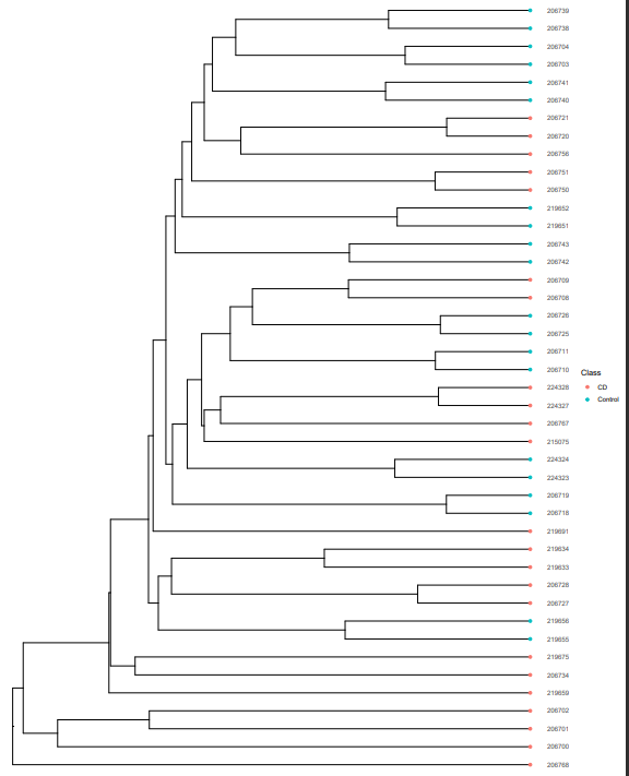
Hierarchical cluster analysis
サンプル間の距離を用いて階層クラスター解析を行い、サンプルの非類似度を推定します。正直この解析のことはよくわかりません。
mpse %<>% mp_cal_clust( .abundance = hellinger, distmethod = "bray", hclustmethod = "average", action = "add" )
# "average", # (UPGAE)
# action = "add" # action is used to control which result will be returned
# The result was added to the internal attributes of the object
It can be extracted via object %>% mp_extract_internal_attr(name='SampleClust') !

# 結果を抽出し、格納
# action = 'add'の場合、hierarchical cluster 解析の結果がMPSE データに追加されるため、この結果を mp_extract_internal_attr コマンドで抽出する
sample.clust <- mpse %>% mp_extract_internal_attr(name='SampleClust')

# The object contained internal attribute: PCoA ADONIS SampleClust

# この結果はggtree によって可視化可能
library(ggtree)
p <- ggtree(sample.clust) + geom_tippoint(aes(color=Class)) + geom_tiplab(as_ylab = TRUE) + ggplot2::scale_x_continuous(expand=c(0, 0.01))

# 図の保存
ggsave("hierarchical_cluster.pdf", plot = p, dpi = 100, width = 12, height = 15, limitsize = FALSE)
階層クラスターの結果と特定の分類レベルの存在量を同時に表示する
library(ggtreeExtra)
library(ggplot2)
phyla.tb <- mpse %>% mp_extract_abundance(taxa.class=Phylum, topn=30)
# The abundance of each samples is nested, it can be flatted using the unnest of tidyr.
phyla.tb %<>% tidyr::unnest(cols=RareAbundanceBySample) %>% dplyr::rename(Phyla="label")
# The abundance of each samples is nested, it can be flatted using the unnest of tidyr.
phyla.tb %<>% tidyr::unnest(cols=RareAbundanceBySample) %>% dplyr::rename(Phyla="label")
ggtreeExtra v1.8.1 For help:
https://yulab-smu.top/treedata-book/
If you use the ggtree package suite in published research, please cite
the appropriate paper(s):
S Xu, Z Dai, P Guo, X Fu, S Liu, L Zhou, W Tang, T Feng, M Chen, L
Zhan, T Wu, E Hu, Y Jiang, X Bo, G Yu. ggtreeExtra: Compact
visualization of richly annotated phylogenetic data. Molecular Biology
and Evolution. 2021, 38(9):4039-4042. doi: 10.1093/molbev/msab166
図示
p1 <- p + geom_fruit( data=phyla.tb, geom=geom_col, mapping = aes(x = RelRareAbundanceBySample, y = Sample, fill = Phyla ), orientation = "y", pwidth = 3, axis.params = list(axis = "x", title = "The relative abundance of phyla (%)", title.size = 4, text.size = 2, vjust = 1), grid.params = list() )
 #offset = 0.4
# 警告メッセージ:
The following column names/name: Class are/is the same to tree data,
the tree data column names are : label, Class, RareAbundanceRarecurve,
Observe, Chao1, ACE, Shannon, Simpson, Pielou, bray, PCo1 (13.59%),
PCo2 (8.59%), PCo3 (7.92%), y, angle.

# 図の保存
ggsave("hierarchical_cluster_Phylum_abundance.pdf", plot = p1, dpi = 100, width = 16, height = 12, limitsize = FALSE)

Biomarker discovery
ここではLEfSe (Nicola Segata and Huttenhower 2011) のような存在量の差分解析(mp_diff_analysis)をやっていきます。
MicrobaiotaProcess 論文によると以下のような結果を残している解析のようです。
Potential disease microbiota biomarkers or probiotic microbiota can be detected by differential abundance analysis. Although there are many tools available, it remains challenging to obtain a good false-positive control.34 To identify the more conservative differential taxa, we developed mp_diff_analysis. We found our method can limit the false positive rate with a better balance of type I and type II errors when compared with metagenomeSeq,35 LEfSe,36 ANCOMBC,37 LinDA,38 and ZicoSeq39 in different datasets simulated from log-normal and normal distributions with different means and standard deviations (Figures SB.3–SB.12).
first test ですべての特徴量について、異なるクラスの値が異なって分布しているかどうかを検定します。つぎに、first test で有意に異なる特徴量について、second test で異なるクラスのサブクラス間のすべてのペアワイズ比較が、クラスのトレンドと明確に一致するかどうかをテストします(ここがよくわかっていません)。
最後に、有意に識別性の高い特徴量はLDA (線形判別分析) またはrf (randomForest) によって評価します。
mp_diff_analysis は2つのステップのtest method を使う側が設定できるので柔軟であると述べられているのですが、使う側が検定を指定できることが良いことなのかわたしにはよくわかりません。結果はtreedataオブジェクトに格納されます。
先にパッケージの読み込みを行います。今回はたくさんあります。
また、この解析はすごく重くて、わたしの場合、ローカルではR studio が落ちまくって話になりませんでした。
必要なパッケージの読み込み
library(ggtree)
library(ggtreeExtra)
library(ggplot2)
library(MicrobiotaProcess)
library(tidytree)
library(ggstar)
library(forcats)
mp_diff_analysis
mpse %<>% mp_diff_analysis( .abundance = RelRareAbundanceBySample, .group = Class, first.test.alpha = 0.01 )

# first test method のデフォルトは"kruskal.test"
# 変えたい場合にはfirst.test.method = glm のようにオプションを指定
# first.test.method の種類:"kruskal.test", "oneway.test", "lm", "glm", or "glm.nb", "kruskal_test", "oneway_test" of "coin"
# 参考:https://rdrr.io/github/YuLab-SMU/MicrobiotaProcess/man/mp_diff_analysis-methods.html
# 結果は taxatree または otutree スロットに格納される
# mp_extract_tree は特定のスロットを抽出する際に使用
taxa.tree <- mpse %>% mp_extract_tree(type="taxatree")
taxa.tree
'treedata' S4 object'.
...@ phylo:
Phylogenetic tree with 1251 tips and 640 internal nodes.
Tip labels:
  OTU_1333, OTU_1005, OTU_1190, OTU_1035, OTU_1525, OTU_1149, ...
Node labels:
  r__root, k__Bacteria, k__Archaea, p__[Thermi], p__Acidobacteria,
p__Actinobacteria, ...
Rooted; no branch lengths.
with the following features available:
  'nodeClass', 'nodeDepth', 'LDAupper', 'LDAmean', 'LDAlower', 'Sign_Class',
'pvalue', 'fdr', 'RareAbundanceBySample', 'RareAbundanceByClass',
'LDAupper.y', 'LDAmean.y', 'LDAlower.y', 'Sign_Class.y', 'pvalue.y', 'fdr.y'.
# The associated data tibble abstraction: 1,891 × 19
# The 'node', 'label' and 'isTip' are from the phylo tree.
    node label    isTip nodeClass nodeDepth LDAupper LDAmean LDAlower Sign_Class
   <dbl> <chr>    <lgl> <chr>         <dbl>    <dbl>   <dbl>    <dbl> <chr>
 1     1 OTU_1333 TRUE  OTU               8       NA      NA       NA NA
 2     2 OTU_1005 TRUE  OTU               8       NA      NA       NA NA
 3     3 OTU_1190 TRUE  OTU               8       NA      NA       NA NA
 4     4 OTU_1035 TRUE  OTU               8       NA      NA       NA NA
 5     5 OTU_1525 TRUE  OTU               8       NA      NA       NA NA
 6     6 OTU_1149 TRUE  OTU               8       NA      NA       NA NA
 7     7 OTU_522  TRUE  OTU               8       NA      NA       NA NA
 8     8 OTU_1063 TRUE  OTU               8       NA      NA       NA NA
 9     9 OTU_215  TRUE  OTU               8       NA      NA       NA NA
10    10 OTU_784  TRUE  OTU               8       NA      NA       NA NA
# ℹ 1,881 more rows
# ℹ 10 more variables: pvalue <dbl>, fdr <dbl>, RareAbundanceBySample <list>,
#   RareAbundanceByClass <list>, LDAupper.y <dbl>, LDAmean.y <dbl>,
#   LDAlower.y <dbl>, Sign_Class.y <chr>, pvalue.y <dbl>, fdr.y <dbl>
# ℹ Use `print(n = ...)` to see more rows
# 異なる分析結果のtibble を抽出する場合
taxa.tree %>% select(label, nodeClass, LDAupper, LDAmean, LDAlower, Sign_Class, pvalue, fdr) %>% dplyr::filter(!is.na(fdr))

# A tibble: 1,856 × 8
   label    nodeClass LDAupper LDAmean LDAlower Sign_Class pvalue   fdr
   <chr>    <chr>        <dbl>   <dbl>    <dbl> <chr>       <dbl> <dbl>
 1 OTU_1333 OTU             NA      NA       NA NA          0.351 0.424
 2 OTU_1005 OTU             NA      NA       NA NA          0.125 0.424
 3 OTU_1190 OTU             NA      NA       NA NA          0.284 0.424
 4 OTU_1035 OTU             NA      NA       NA NA          0.351 0.424
 5 OTU_1525 OTU             NA      NA       NA NA          0.351 0.424
 6 OTU_1149 OTU             NA      NA       NA NA          0.351 0.424
 7 OTU_522  OTU             NA      NA       NA NA          0.615 0.681
 8 OTU_1063 OTU             NA      NA       NA NA          0.284 0.424
 9 OTU_215  OTU             NA      NA       NA NA          0.130 0.424
10 OTU_784  OTU             NA      NA       NA NA          0.125 0.424
# ℹ 1,846 more rows
# ℹ Use `print(n = ...)` to see more rows
taxa.tree の中身
'treedata' S4 object'.
...@ phylo:
Phylogenetic tree with 1251 tips and 640 internal nodes.
Tip labels:
  OTU_1333, OTU_1005, OTU_1190, OTU_1035, OTU_1525, OTU_1149, ...
Node labels:
  r__root, k__Bacteria, k__Archaea, p__[Thermi], p__Acidobacteria,
p__Actinobacteria, ...
Rooted; no branch lengths.
with the following features available:
  'nodeClass', 'nodeDepth', 'RareAbundanceBySample', 'RareAbundanceByClass',
'LDAupper', 'LDAmean', 'LDAlower', 'Sign_Class', 'pvalue', 'fdr'.
# The associated data tibble abstraction: 1,891 × 13
# The 'node', 'label' and 'isTip' are from the phylo tree.
    node label    isTip nodeClass nodeDepth RareAbundanceBySample
   <dbl> <chr>    <lgl> <chr>         <dbl> <list>
 1     1 OTU_1333 TRUE  OTU               8 <tibble [43 × 4]>
 2     2 OTU_1005 TRUE  OTU               8 <tibble [43 × 4]>
 3     3 OTU_1190 TRUE  OTU               8 <tibble [43 × 4]>
 4     4 OTU_1035 TRUE  OTU               8 <tibble [43 × 4]>
 5     5 OTU_1525 TRUE  OTU               8 <tibble [43 × 4]>
 6     6 OTU_1149 TRUE  OTU               8 <tibble [43 × 4]>
 7     7 OTU_522  TRUE  OTU               8 <tibble [43 × 4]>
 8     8 OTU_1063 TRUE  OTU               8 <tibble [43 × 4]>
 9     9 OTU_215  TRUE  OTU               8 <tibble [43 × 4]>
10    10 OTU_784  TRUE  OTU               8 <tibble [43 × 4]>
# ℹ 1,881 more rows
# ℹ 7 more variables: RareAbundanceByClass <list>, LDAupper <dbl>,
#   LDAmean <dbl>, LDAlower <dbl>, Sign_Class <chr>, pvalue <dbl>, fdr <dbl>
# ℹ Use `print(n = ...)` to see more rows
taxa.tree の可視化 (上手くいきませんでした)
p1 <- ggtree( taxa.tree, layout="radial", size = 0.3 ) + geom_point( data = td_filter(!isTip), fill="white", size=1, shape=21 )

# 門を強調する
p2 <- p1 + geom_hilight( data = td_filter(nodeClass == "Phylum"), mapping = aes(node = node, fill = label) )
# 自分のデータでやったときは出なかったのですが、「x$node != rn で: 長いオブジェクトの長さが短いオブジェクトの長さの倍数になっていません」というエラーが出てしまったので、以下のように変更しました。
filtered_data <- taxa.tree@data %>% filter(!is.na(nodeClass))
filtered_data <- na.omit(filtered_data)
filtered_data <- filtered_data[1:nrow(p1$data), ]
p2 <- p1 + geom_hilight( data = filter(filtered_data, nodeClass == "Phylum")[1:nrow(p1$data), ], mapping = aes(node = node, fill = label) )
#filtered_data[1:nrow(p1$data), ]は、filtered_dataの行数をp1$dataの行数に制約するために使用されています。1:nrow(p1$data)は、p1$dataの行数に対応する行インデックスを生成します。それにより、filtered_dataの行数がp1$dataの行数に制約され、二つのデータフレームの行数を一致させることができます。(これでいいのかは不明)

# 特徴量 (OTU) の相対量を表示
p3 <- p2 + ggnewscale::new_scale("fill") + geom_fruit( data = td_unnest(RareAbundanceBySample), geom = geom_star, mapping = aes( x = fct_reorder(Sample, Class, .fun=min), size = RelRareAbundanceBySample, fill = Class, subset = RelRareAbundanceBySample > 0 ), starshape = 13, starstroke = 0.25, offset = 0.04, pwidth = 0.8, grid.params = list(linetype=2) ) + scale_size_continuous( name="Relative Abundance (%)", range = c(.5, 3) ) + scale_fill_manual(values=c("#1B9E77", "#D95F02"))

# ツリーにtip label を表示
p4 <- p3 + geom_tiplab(size=2, offset=7.2)

# 有意なOTUのLDAを表示
p5 <- p4 + ggnewscale::new_scale("fill") + geom_fruit( geom = geom_col, mapping = aes( x = LDAmean, fill = Sign_Class, subset = !is.na(LDAmean) ), orientation = "y", offset = 0.3, pwidth = 0.5, axis.params = list(axis = "x", title = "Log10(LDA)", title.height = 0.01, title.size = 2, text.size = 1.8, vjust = 1), grid.params = list(linetype = 2) )

# kruskal.testの後にFDR が有意な分類群を表示する(デフォルト)
p6 <- p5 + ggnewscale::new_scale("size") + geom_point( data=td_filter(!is.na(Sign_Class)), mapping = aes(size = -log10(fdr), fill = Sign_Class, ), shape = 21, ) + scale_size_continuous(range=c(1, 3)) + scale_fill_manual(values=c("#1B9E77", "#D95F02"))

plot <- p6 + theme( legend.key.height = unit(0.3, "cm"), legend.key.width = unit(0.3, "cm"), legend.spacing.y = unit(0.02, "cm"), legend.text = element_text(size = 7), legend.title = element_text(size = 9), )

ggsave("diff-species_abundance-sample.pdf", plot = plot, dpi = 100, width = 16, height = 12, limitsize = FALSE)
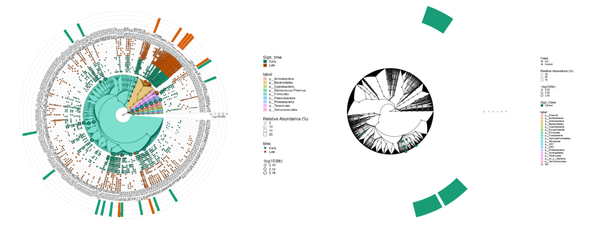
差分解析(mp_diff_analysis)の結果の図示
特に指定しない場合には門レベルの結果が出るようです。
p <- mpse %>% mp_plot_diff_res( group.abun = TRUE, pwidth.abun=0.1 ) + scale_fill_manual(values=c("deepskyblue", "orange")) + scale_fill_manual( aesthetics = "fill_new", values = c("orange", "deepskyblue") ) + scale_fill_manual( aesthetics = "fill_new_new", values = c("#E41A1C", "#377EB8", "#4DAF4A", "#984EA3", "#FF7F00", "#FFFF33", "#A65628", "#F781BF", "#999999", "#66C2A5", "#FC8D62", "#8DA0CB", "#E78AC3", "#A6D854", "#FFD92F", "#E5C494", "#B3B3CC"))

### オプションなどの説明
# group.abun はサンプルの代わりにグループの相対量を表示するかどうかを指定するオプションでデフォルトはFALSE
# scale_fill_manual( aesthetics = "fill_new", values = c("deepskyblue", "orange") ) はグループの塗分けなので、今回は二色
# scale_fill_manual( aesthetics = "fill_new_new", values = c("#E41A1C", "#377EB8", "#4DAF4A", "#984EA3", "#FF7F00", "#FFFF33", "#A65628", "#F781BF", "#999999", "#66C2A5", "#FC8D62", "#8DA0CB", "#E78AC3", "#A6D854", "#FFD92F", "#E5C494", "#B3B3CC")) は有意差のあった
# 指定するカラー数は有意にが何種類出てくるかによって変える
# 有意なグループ数に対して指定カラー数が少ないとエラーが出る

# 図の保存
ggsave("diff-species_abundance-sample.pdf", plot = p, dpi = 100, width = 16, height = 12, limitsize = FALSE)
おまけ:網(class)についてだけ抽出して書きたい場合
.taxa.class = Classp <- mpse %>% mp_plot_diff_res( group.abun = TRUE, pwidth.abun=0.1, .taxa.class = Class ) + scale_fill_manual(values=c("deepskyblue", "orange")) + scale_fill_manual( aesthetics = "fill_new", values = c("deepskyblue", "orange") ) + scale_fill_manual( aesthetics = "fill_new_new", values = c("#1f77b4", "#ff7f0e", "#2ca02c", "#d62728", "#9467bd", "#8c564b", "#e377c2", "#7f7f7f", "#bcbd22", "#17becf", "#393b79", "#637939", "#8c6d31", "#843c39", "#7b4173", "#5254a3", "#637939", "#8c6d31", "#843c39", "#7b4173", "#5254a3", "#637939", "#8c6d31", "#843c39", "#7b4173", "#5254a3", "#637939", "#8c6d31", "#843c39", "#7b4173", "#5254a3", "#637939", "#8c6d31", "#843c39", "#7b4173"))
# 図の保存
ggsave("diff-Class_abundance-sample.pdf", plot = p, dpi = 100, width = 16, height = 12, limitsize = FALSE)

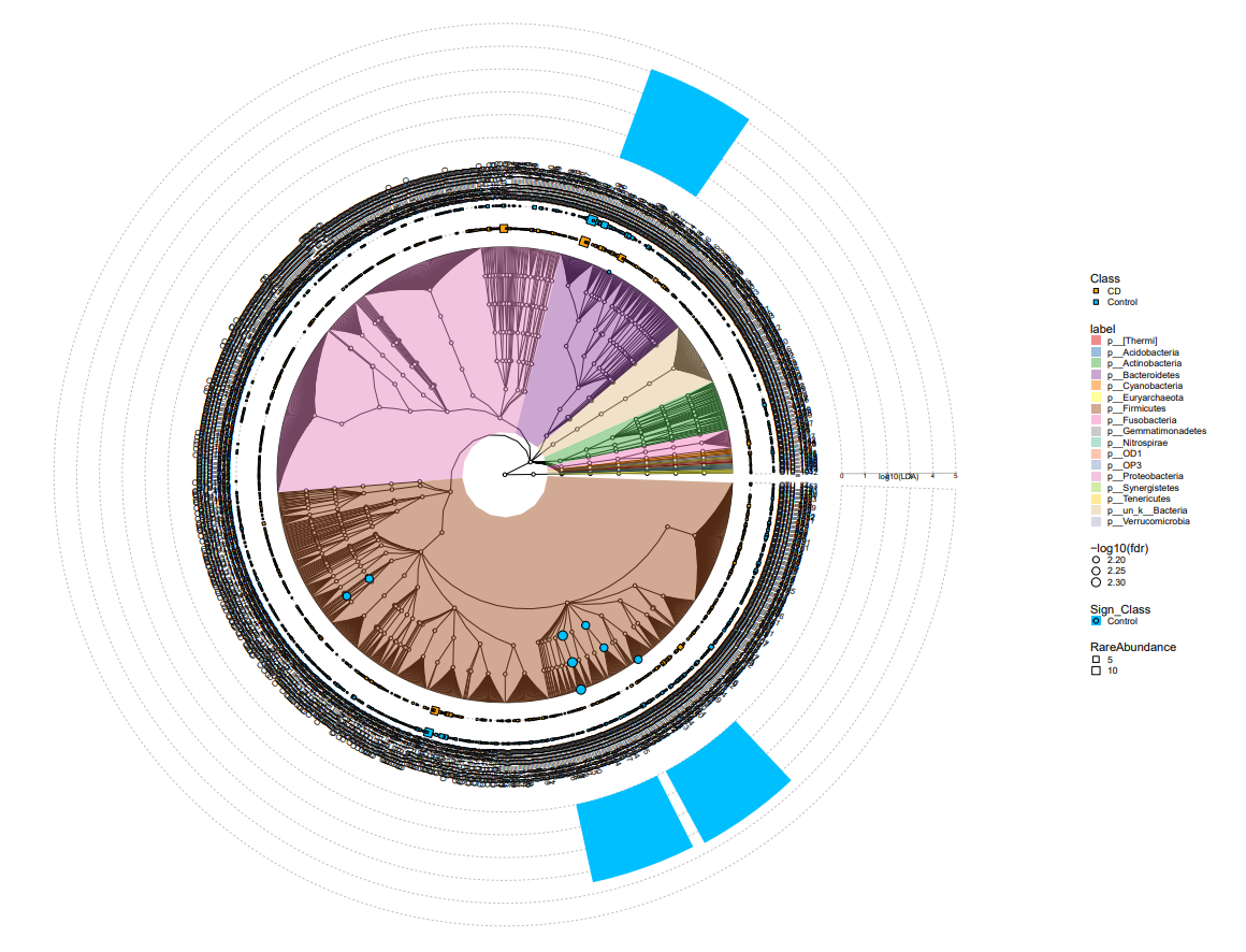
クラドグラム(cladogram)の描画
f <- mpse %>% mp_plot_diff_cladogram( label.size = 2.5, hilight.alpha = .3, bg.tree.size = .5, bg.point.size = 2, bg.point.stroke = .25 ) + scale_fill_diff_cladogram( values = c('deepskyblue', 'orange') ) + scale_size_continuous(range = c(1, 4))

# 図の保存
ggsave("cladogram_diff_species.pdf", plot = f, dpi = 100, width = 16, height = 12, limitsize = FALSE)

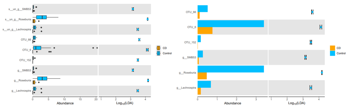
LDA 効果量とabundance をボックスプロットとして図示
f.box <- mpse %>% mp_plot_diff_boxplot( .group = Class, ) %>% set_diff_boxplot_color( values = c("orange", "deepskyblue"), guide = guide_legend(title=NULL) )

f.bar <- mpse %>% mp_plot_diff_boxplot( taxa.class = c(Genus, OTU), group.abun = TRUE, removeUnknown = TRUE, ) %>% set_diff_boxplot_color( values = c("orange", "deepskyblue"), guide = guide_legend(title=NULL) )

# オプションの説明
# taxa.class = c(Genus, OTU), # select the taxonomy level to display
# group.abun = TRUE, # display the mean abundance of each group
# removeUnknown = TRUE, # whether mask the unknown taxa.

plot <- aplot::plot_list(f.box, f.bar)

# 図の保存
ggsave("abundance_LDA-effect-size_diff-taxa.pdf", plot = plot, dpi = 100, width = 16, height = 5, limitsize = FALSE)
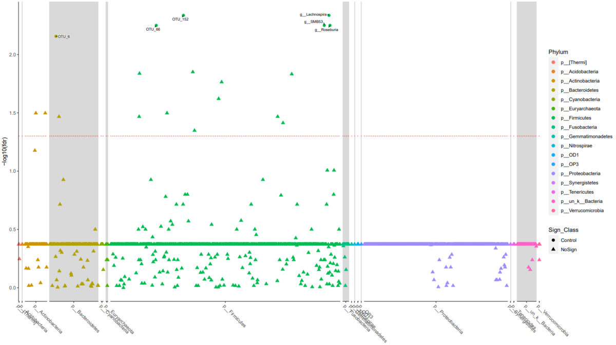
LDA 効果量とabundance をマンハッタンプロットとして図示
f.mahattan <- mpse %>% mp_plot_diff_manhattan( .group = Sign_Class, .y = fdr, .size = 2.4, taxa.class = c('OTU', 'Genus'), anno.taxa.class = Phylum )

# 図の保存
ggsave("mahattanplot_diff-taxa.pdf", plot = f.mahattan, dpi = 100, width = 16, height = 9, limitsize = FALSE)
今回はここまでです!お疲れさまでした~